Raytracing Intersections: The Plane
The humble plane, a flat, infinitely thin surface that extends infinitely. It might not seem much, but it’s used everywhere for ray-intersections, from AABBs, to voxels, triangle meshes, BVHs, convex polyhedrons and many more. One could even say it is the building block of raytracing.
Today, we will derive an intersection of a ray with a plane, and then build up to its applications in the subsequent posts.
Derivation
A ray can be defined as its origin $ O $, unit direction $ \hat D $, and the ray parameter $ t $, which is the distance to get to our intersection point $ P $, and what we are trying to solve:
\[P = O + \hat D t\]There are two ways we can derive the intersection of a ray and a plane, algebraically and geometrically. The former is quite straightforward, but the latter may provide us with some insight on how it works.
Algebraic derivation
The plane equation is defined as such:
\[P \cdot \hat N = d\]where $ P $ is any point, $ N $ the unit normal of the plane, and $ d $ the signed distance of $ P $ to the plane. When $ d = 0 $, $ P $ lies exactly on the plane.
To get the interesction of the ray to the plane, we substitute the ray equation into the plane equation and solve for $ t $:
\[(O + \hat D t) \cdot \hat N = 0\]We can separate the terms inside the dot product using the distributive and the scalar multiplication property of the dot product1:
\[O \cdot \hat N + \hat D t \cdot \hat N = 0\] \[O \cdot \hat N + (\hat D \cdot \hat N)t = 0\]Rearranging the terms to get $ t $, we then get our solution:
\[t = -\frac {O \cdot \hat N} {\hat D \cdot \hat N}\]Geometric derivation
The derivation above is straightforward, but it didn’t really quite tell us how it works. The geometric derivation on the other hand can give us insights using some properties of the dot product.
Below we can see how the intersection of the ray and the plane in 2D:
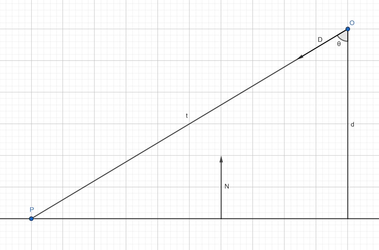
 Ray-plane interesction diagram in 2D
We know from trigonometry that:
\[\cos(\theta) = \frac {\mathrm {adjacent}} {\mathrm {hypotenuse}}\]We are solving for the hypotenuse which is $ t $, and the adjacent being $ d $:
\[\mathrm {hypotenuse} = \frac {\mathrm {adjacent}} {\cos(\theta)}\] \[t = \frac {d} {\cos(\theta)}\]The dot product is defined as such:
\[A \cdot B = \cos(\theta) ~ |A| ~ |B|\]When one of the vector is of unit length, the result of their dot product is a scalar projection2 of $ A $ along $ \hat B $:
\[A \cdot \hat B = \cos(\theta) ~ |A|\]From it, we can compute the adjacent $ d $ from the ray position $ O $ and the normal $ N $:
\[O \cdot \hat N = d\]The result of the dot product of two unit vectors is the cosine of the angle between them:
\[\hat A \cdot \hat B = \cos(\theta)\]Therefore, we take the dot product of the ray direction and the normal, with the result negated as they are pointing away from each other:
\[-\hat D \cdot \hat N = \cos(\theta)\]Putting everything together, we get our solution as before:
\[t = -\frac {O \cdot \hat N} {\hat D \cdot \hat N}\]Usage
In code our formula looks like so, we also add a check when there is no intersection, which is when $ t < 0 $ :
1
2
3
4
5
6
7
float rayPlaneIntersection(vec3 rayOrigin, vec3 rayDir, vec3 normal) {
    float t = -dot(rayOrigin, normal) / dot(rayDir, normal);
    if (t < 0.0) {
        return MAX_DISTANCE; // No hit
    }
    return t;
}
To get our hit position, we simply take our ray parameter and plug it in the ray equation:
1
2
float t = rayPlaneIntersection(rayOrigin, rayDir, planeNormal);
vec3 position = rayOrigin + rayDir * t;
Notes
We can detect when the ray does not intersect the plane when both the ray origin is outside the plane $ O \cdot \hat N > 0 $ and the ray direction is pointing away from it $ \hat D \cdot \hat N > 0 $, or the ray origin is inside plane $ O \cdot \hat N < 0 $ and the ray direction is pointing away from it $ \hat D \cdot \hat N < 0 $. This check simplifies to $ t < 0 $ as seen from the code above.
We can tell what side of the plane we are interescting from the sign of the dot product of the ray direction and the normal. If $ D \cdot \hat N $ is $ < 0 $, then we are intersecting the front face, otherwise the back face.
If the normal $ \hat N $ is axis aligned, the dot product would be simplified to a selection of a component of the vector with the normal’s axis, e.g.:
- The formula above is for a plane that is located at the origin. To translate the plane at position $ Q $, we can subtract it to the ray origin to get a plane located at $ Q $:
- Alternatively, we can translate the plane using a scalar $ d $ instead, where $ d $ can be thought of as the plane distance from the origin along $ \hat N $:
The derivation above assume that the normal is a unit/normalized vector for simplicity, but the formula also works when the normal is unnormalized. This is due to its length canceling out as they appear in the numerator and denominator.
Substituting the unnormalized normal $ \vec N $ as the normalized vector multiplied by its length $ \vec N = k \hat N $:
If the ray direction is also unnormalized, its length $ k $ would cancel out during the ray equation. Do note though that the resulting ray parameter $ t $ would be scaled by its inverse length $ \frac{1}{k} $. This might be an issue when you are using the ray parameter for something that requires its actual length.
Substituting the unnormalized ray direction as $ \vec D = k \hat D $ in both the ray and plane equations:
As we have seen, there is quite a bit more to planes as simple as they seems.
Stay tuned on the next part where we extend this using multiple planes to intersect boxes. Seeya! 🐸